Acoustic analysis pt. 2

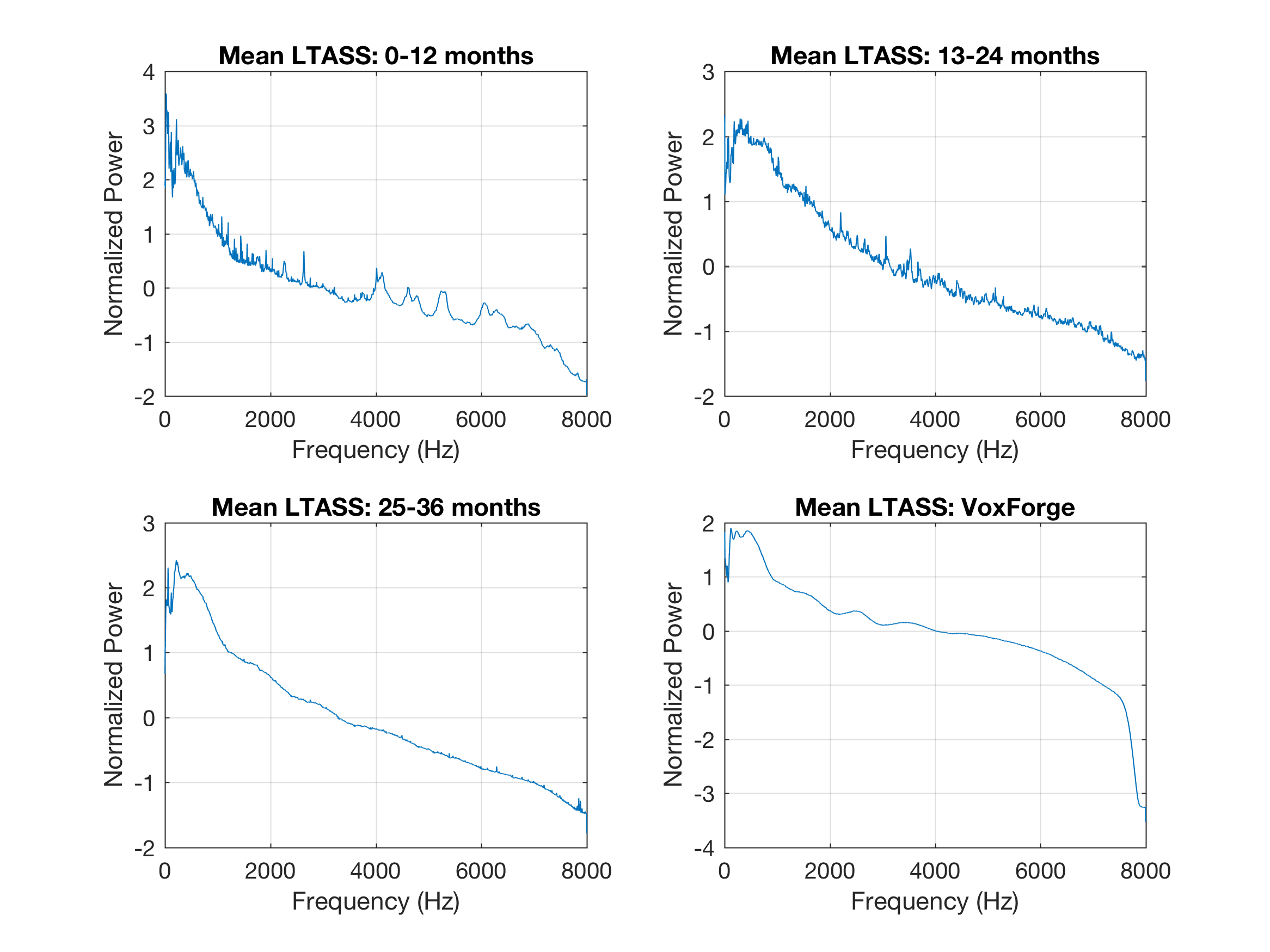
This week I worked on comparing the mean power spectral density estimates (PSDs or mean LTASS) results of the three age ranges and the VoxForge corpus. The goal is to observe how the acoustics (spectrum) characteristics change across the ages and highlight any spectral patterns or structures that are similar to the VoxForge data.

Note: Here, mean PSD and mean LTASS are interchangeable

Graphing spectrums

.
.
.
% Group mean PSDs
dataMean = [childes1_mean, childes2_mean, childes3_mean, voxforge_mean];

% Set x-axis
ff = 0:1/2049:1-(1/2049);
x = 8000.*ff;

% Graph individual average PSDs(mean LTASS)
figure
subplot(2,2,1)
plot(x,dataMean(:,1))
title('Mean LTASS: 0-12 months')
xlabel('Frequency (Hz)')
ylabel('Normalized Power')
grid on
subplot(2,2,2)
plot(x,dataMean(:,2))
title('Mean LTASS: 13-24 months')
xlabel('Frequency (Hz)')
ylabel('Normalized Power')
grid on
subplot(2,2,3)
plot(x,dataMean(:,3))
title('Mean LTASS: 25-36 months')
xlabel('Frequency (Hz)')
ylabel('Normalized Power')
grid on
subplot(2,2,4)
plot(x,dataMean(:,4))
title('Mean LTASS: VoxForge')
xlabel('Frequency (Hz)')
ylabel('Normalized Power')
grid on

% Graph grouped average PSDs
figure
plot(x,dataMean(:,1),x,dataMean(:,2),x,dataMean(:,3),x,dataMean(:,4))
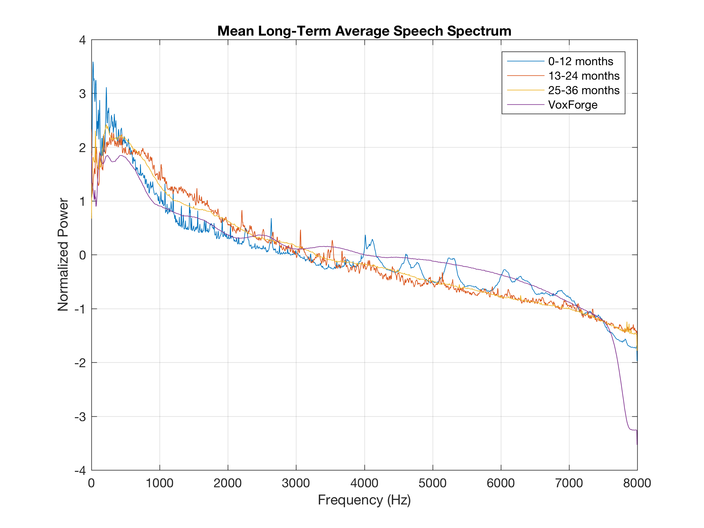
title('Mean Long-Term Average Speech Spectrum')
xlabel('Frequency (Hz)')
ylabel('Normalized Power')
legend('0-12 months','13-24 months','25-36 months','VoxForge')
grid on

Comparing frequency components

Using the above graphs, I wanted to look at the frequency components shared (or not shared) across the spectrums:

% Find prominent peaks in spectra
[pk1,lc1] = findpeaks(dataMean(:,1),'SortStr','descend','NPeaks',100);
[pk2,lc2] = findpeaks(dataMean(:,2),'SortStr','descend','NPeaks',100);
[pk3,lc3] = findpeaks(dataMean(:,3),'SortStr','descend','NPeaks',100);
[pk4,lc4] = findpeaks(dataMean(:,4),'SortStr','descend','NPeaks',100);
P1peakFreqs = x(lc1); P2peakFreqs = x(lc2); P3peakFreqs = x(lc3); P4peakFreqs = x(lc4);

% Set x-axis
NPeaks = 1:1:100;

% Graph prominent peaks (local maximums)
figure
plot(NPeaks,P1peakFreqs,NPeaks,P2peakFreqs,NPeaks,P3peakFreqs,NPeaks,P4peakFreqs);
title('Most Prominent Frequency Components')
xlabel('Peak Number')
ylabel('Frequency (Hz)')
legend('0-12 months','13-24 months','25-36 months','VoxForge','Location','northwest')
grid on

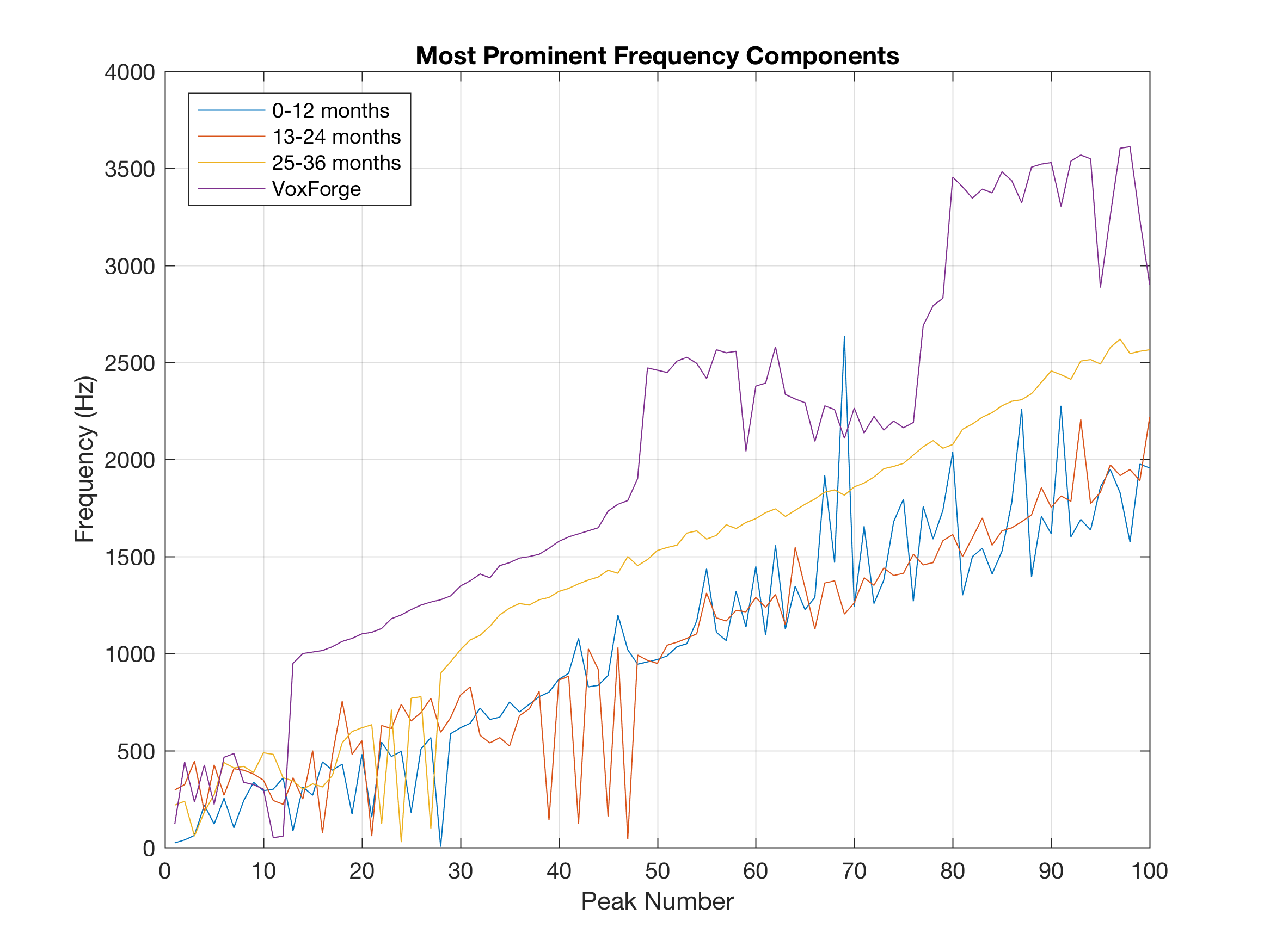
The graph above shows 100 local maximum (frequency components with significant energy) across each spectrum.

Signal-to-noise ratio

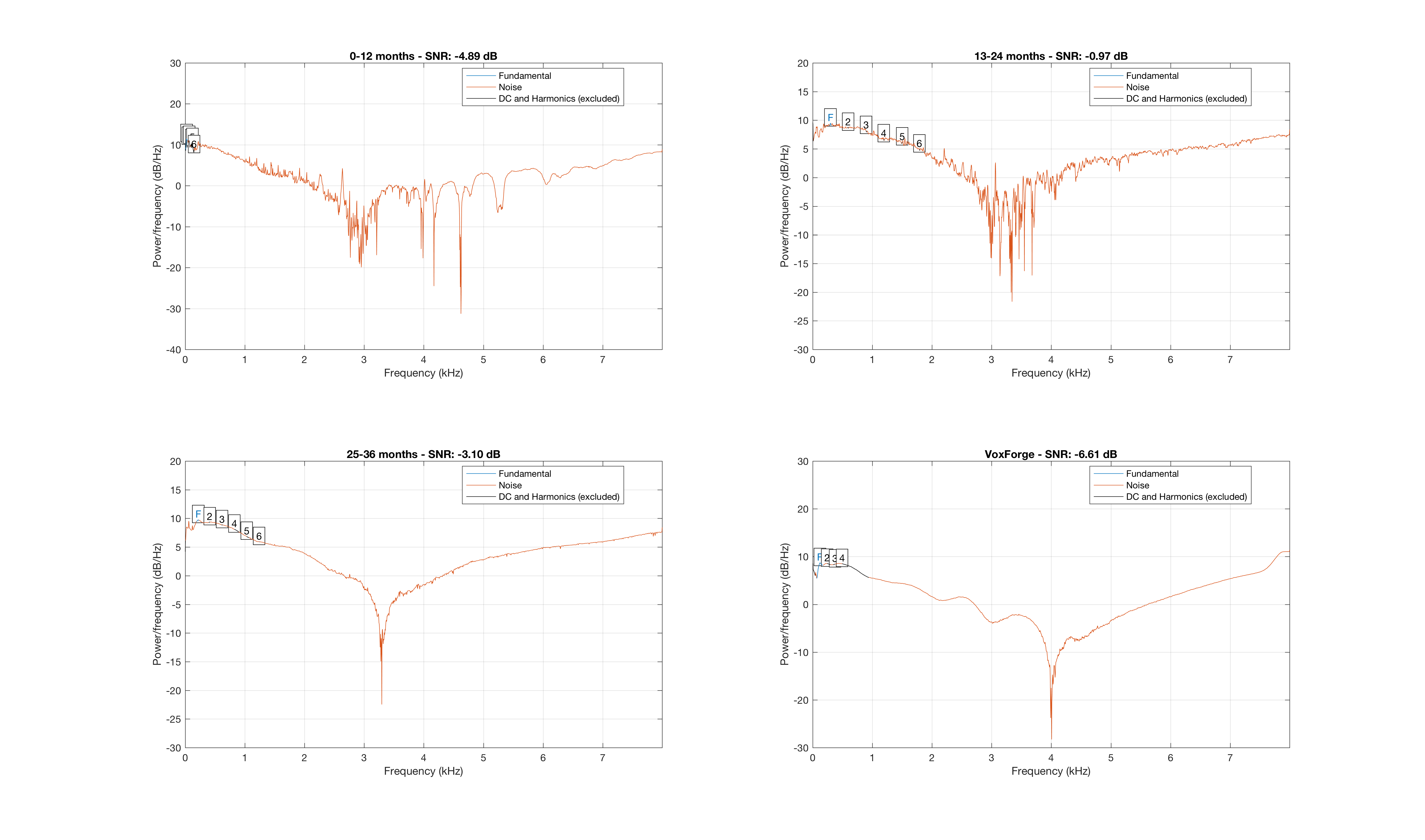
Then, I wanted to use signal-to-noise ratio (snr) of the one-sided PSDs to understand how snr of the spectrums differ. In particular, how the noise differs across the spectrums.

In general, snr values depend on the application domain. That is, concluding anything from snr values alone (particularly because we’re looking at average spectrums and not single audio files) would be misleading. Nevertheless, we’re interested in training a speech recognition system, and according to the “Audio Handbook” by Gordon J King, the differences between whispering and “moderate” speech is greater than 20 dB. Further, many people consider snr values greater than 30 dB to be “clean speech”.

Note: I tried previously to collect average snr values over the different corpora, but those results didn’t seem to be very informative.

% Graph snr using PSD
figure
subplot(2,2,1)
snr(dataMean(:,1),x,'psd')
subplot(2,2,2)
snr(dataMean(:,2),x,'psd')
subplot(2,2,3)
snr(dataMean(:,3),x,'psd')
subplot(2,2,4)
snr(dataMean(:,4),x,'psd')

Structural similarity index

In looking for interesting and useful ways to compare the mean LTASS of the four corpora I found structural similarity (SSIM) index. SSIM is used for measuring the perceived quality or similarity between two images. SSIM is supposed to be an “improvement” on traditional methods like peak signal-to-noise ratio (psnr) and mean squared error (MSE).

MATLAB has a ssim function for measuring image quality. The interface was simple enough, so I wanted to try applying it to the LTASS results. Of course, instead of comparing one image (or array of pixels) to a referenced image, I will compare spectrums (array of power by frequency bins) to a referenced spectrum:

% Use structural similarity index (ssim) to asses quality of spectras against each other
ssim_table = zeros(4,4);
for i = 1:4
    for j = 1:4
    ssim_table(i,j) = ssim(dataMean(:,i),dataMean(:,j));
    end
end

MATLAB output:

                 0-12 months    13-24 months    25-36 months    VoxForge
                 ___________    ____________    ____________    _________

    0-12 months            1         0.38436         0.53506      0.38614
    13-24 months     0.38436               1         0.53862      0.37479
    25-36 months     0.53506         0.53862               1      0.60044
    VoxForge         0.38614         0.37479         0.60044            1

Correlation

Additionally, we can do a linear correlation between the four spectras:

ssim_table = corr(meanData);

MATLAB output:

                 0-12 months    13-24 months    25-36 months    VoxForge
                 ___________    ____________    ____________    _________

   0-12 months             1         0.93996         0.95871      0.91284
   13-24 months      0.93996               1         0.99175        0.895
   25-36 months      0.95871         0.99175               1       0.9085
   VoxForge          0.91284           0.895          0.9085            1

Both the ssim and corr results are something to ponder about. We find that the ssim of the other spectras are most “structurally similar” to the 25-36 month age range (0.53506, 0.53862, 0.60044), where the VoxForge spectra is the most structurally similar (0.6004) and the 13-24 month age range is least structurally similar (0.37479). Further, the four spectras are all highly correlated, which is to be expected. 0-12 month age range is most correlated with the 25-36 month age range (0.95871), and the VoxForge spectra is most correlated with the 0-12 month age range spectra (0.91284). Again, we’re not sure how significant these resultd are.

The source of acoustic differences

At the first pass, this was an interesting experiment. There are clear differences between the mean LTASS of the four corpora. Hence, I will continue to spend time digging into particular portions of the spectrum (i.e. voice frequency) to further asses how these acoustics are structured. Additionally, I wonder about the source of these differences. Could the recording quality affect the results? Each subcorpora (researcher) maintains its own method of recording and so some researchers might have used better audio equipment, might be in more controlled environments, etc. In fact, listening to one of the VoxForge recordings and a typical CHILDES recording has prompted me to also consider assessing the acoustics of each subcorpora at some point.

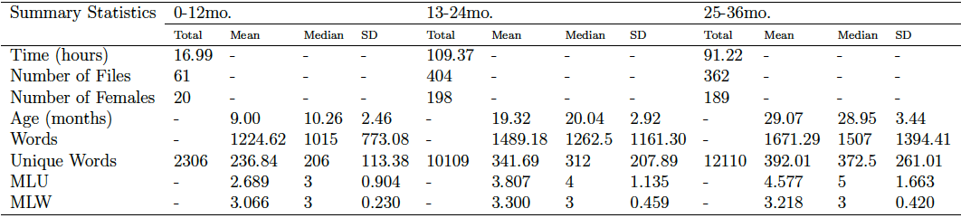
At any rate, below is a table created by Rebekah that summarizes the statistics over the three CHILDES age ranges. At the moment, we don’t have summary statistics for the VoxForge data to compare, but these can help inform new inquiries.

Voice activity detection

It should be noted that the CHILDES audio segments I generated and used for the above acoustic analysis are lacking in comparability. As I mentioned previously, the time stamps I used to extract the audio segments don’t always correspond to speech utterances. To be clear, while the transcribers worked to encode the actual words uttered, the recordings of the actual words are sometimes unclear, noisy, and contain unnecessary silence. This silence, and general noise could have some effect on the LTASS results and will surely effect the recognition results of the ASR system. Hence, there needs to be a way to extract meaningful speech from the audio segments before using it to train the ASR. People typically perform this task using Voice activity detection (VAD) and in truth, I should have applied VAD before segmenting the audio files from the transcripts.

Best,
EO